- Published on
Step by Step machine learning - 4
- Author

- Name
- yceffort
Training Models
정규 방정식을 활용한 선형 회귀
import numpy as np
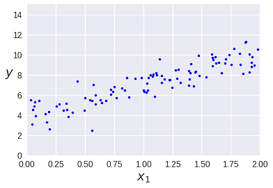
X = 2 * np.random.rand(100, 1)
y = 4 + 3 * X + np.random.randn(100, 1)
테스트 용으로 데이터를 만들어 보겠습니다.
plt.plot(X, y, "b.")
plt.xlabel("$x_1$", fontsize=18)
plt.ylabel("$y$", rotation=0, fontsize=18)
plt.axis([0, 2, 0, 15])
plt.show()
X_b = np.c_[np.ones((100, 1)), X]
theta_best = np.linalg.inv(X_b.T.dot(X_b)).dot(X_b.T).dot(y)
theta_best
array([[4.21509616],
       [2.77011339]])
위에서 로 생성해서 와 를 기대했지만, 실제로는 와 가 나왔다.
이 값을 기반으로 예측을 한번 해보자.
X_new = np.array([[0], [2]])
X_new_b = np.c_[np.ones((2, 1)), X_new]
y_predict = X_new_b.dot(theta_best)
y_predict
array([[ 3.86501051],
       [10.14333409]])
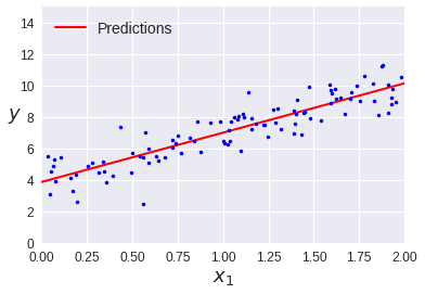
예측한 그래프를 그리자.
plt.plot(X_new, y_predict, "r-", linewidth=2, label="Predictions")
plt.plot(X, y, "b.")
plt.xlabel("$x_1$", fontsize=18)
plt.ylabel("$y$", rotation=0, fontsize=18)
plt.legend(loc="upper left", fontsize=14)
plt.axis([0, 2, 0, 15])
plt.show()
sci-kit learn으로 하면 아래와 같이 간단하게 할 수 있다.
from sklearn.linear_model import LinearRegression
lin_reg = LinearRegression()
lin_reg.fit(X, y)
lin_reg.intercept_, lin_reg.coef_
(array([3.86501051]), array([[3.13916179]]))
lin_reg.predict(X_new)
array([[ 3.86501051],
       [10.14333409]])
Gradient Descent(경사하강법)를 활용한 선형 회귀
eta = 0.1
n_iterations = 1000
m = 100
theta = np.random.randn(2,1)

for iteration in range(n_iterations):
    gradients = 2/m * X_b.T.dot(X_b.dot(theta) - y)
    theta = theta - eta * gradients
theta
X_new_b.dot(theta)
array([[3.86501051],
       [3.13916179]])

array([[ 3.86501051],
       [10.14333409]])
theta_path_bgd = []

def plot_gradient_descent(theta, eta, theta_path=None):
    m = len(X_b)
    plt.plot(X, y, "b.")
    n_iterations = 1000
    for iteration in range(n_iterations):
        if iteration < 10:
            y_predict = X_new_b.dot(theta)
            style = "b-" if iteration > 0 else "r--"
            plt.plot(X_new, y_predict, style)
        gradients = 2/m * X_b.T.dot(X_b.dot(theta) - y)
        theta = theta - eta * gradients
        if theta_path is not None:
            theta_path.append(theta)
    plt.xlabel("$x_1$", fontsize=18)
    plt.axis([0, 2, 0, 15])
    plt.title(r"$\eta = {}$".format(eta), fontsize=16)


np.random.seed(42)
theta = np.random.randn(2,1)  # random initialization

plt.figure(figsize=(10,4))
plt.subplot(131); plot_gradient_descent(theta, eta=0.02)
plt.ylabel("$y$", rotation=0, fontsize=18)
plt.subplot(132); plot_gradient_descent(theta, eta=0.1, theta_path=theta_path_bgd)
plt.subplot(133); plot_gradient_descent(theta, eta=0.5)

plt.show()
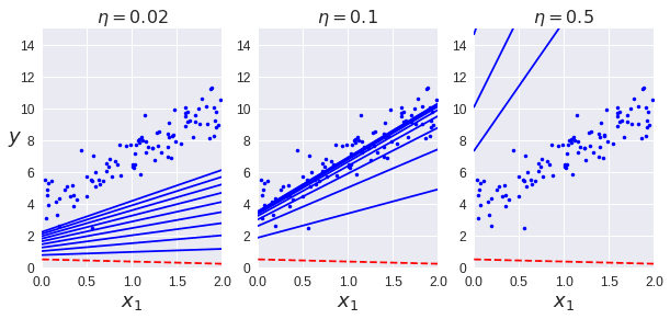
Learning Rate가 너무 작으면 최적의 솔루션을 찾는데 너무 오래 걸리고, 너무 클 경우에는 아예 찾지 못하고 벗어나 버린다.